Roxia AI in Filtration

The step of solid/liquid separation (pressure filtration for the case of this study) is usually one of the last steps in the chain of raw material transformation in concentration plants adding tremendous value to the product being handled. As in every production process, it is expected that the resulting products (cake) comply with a series of prescribed conditions in terms of planned production, operational expenses (resource consumption), and quality.Sound world-class asset management of the solid/liquid separation equipment is key to meet these operative requirements and might well be the difference between reaching budgeted profits or wasting company money continuously. Nonetheless, not even the most rigorous world-class asset management structure can completely foresee the level of impact that deviated process variations in equipment upstream can have on the filtration step. Nor the reactive measures taken by the filtration team can guarantee to compensate for these process deviations in time to keep production, consumables, and quality in the budgeted levels. Filtration units such as pressure filters are provided with rigid settings, a fixed set of stages to be followed or physical conditions to be met during each filtration cycle regardless of the quality of the slurry being fed to the filter. This rigidity makes continued reactive adjustments an untenable endeavor. Constant supervision is needed to manually change these filtration settings to accommodate to slurry conditions to get the best possible output from the filter. Unfortunately, this task is labor-intensive, and having constant supervision plays against the limited organizational structure in place. Many cycles can be run before a suitable action is taken in the filtration settings or ideally before the deviation is corrected in the upstream process. There seems to still prevail an independency of pipelined processes, where changes in key variables are not automatically communicated to the rest of the actors across the production chain introducing thus negative consequences. This paper aims to set the grounds for migrating from a manual and close-to-obsolete filter supervision to a novel automatized adaptive supervision-free response philosophy. Using developments and applications in artificial intelligence algorithms in industrial processes, and data from a filtration process consisting of three pressure filters and their auxiliary equipment in a Zinc concentration plant, it will be shown that optimization algorithms subjected to the operative, resource consumption, and quality constraints are viable to provide key operational information. Information that could be used as feedback to the automation system of the filter originating a new generation of high dynamically adaptable equipment. It is imperative to mention, that the optimization proposed is always paired with the process limitations inherent to the mechanical design of the filter. There are ranges where no optimization or operational parameter adjustment could make the filter output within desired conditions. The scope of this study is framed to that range where an acceptable product might be still viable.

In the solid-liquid separation chain, pressure filtration represents, in many cases, the stage where the process adds tremendous economic value and manageability to the filtration output, the cake. A filter is a simple piece of equipment for a very complicated process [1] . Its operation principle is based on applying pressure on the solid-liquid mixture (slurry), so the excess liquid can be removed through a filter medium [2]. There seems not to be any more science than that. Yet, filter operation can become a headache and even a reason for high penalties to the filter owner when the cake does not meet the required specifications. Not to mention the high economic losses.

A filter under stable process conditions and good maintenance produces cakes that consistently meet the specifications. Under stability, the outcome repeatability is high. This might be why, from the beginning, filter designers and experts have set fixed rules for each of the stages that make up the filtration cycle, the recipe. Over the thousands of filters of this type installed and ever used worldwide, the recipe is handled in the same way: a fixed set of rules that fit stable conditions. However, this utopia is hardly ever the case.

Unfortunately, the filter has limited or no control over the characteristics of the slurry received. Neither the filter can self-adjust to these slurry variations because of the intrinsic nature of the filtration recipe. But why does the slurry quality change? In the simple case, the metallurgy of the processed mineral changes. In a more complicated case, the organizational case, production processes in the same plant are often run as siloed operations.

These siloed operations act as buffers that delay the information flow causing slow reaction times down-stream. When new slurry characteristics are noticed, it is then when production personnel make changes to the recipe to adjust the filter to this new input. The delta between the slurry first changed and the recipe changed is often of a costly magnitude in economic terms. Do not disregard the fact that it might be the case that the slurry, under those conditions, is not processable by the equipment at all. Nor is there the expertise in-house to make appropriate recipe adjustments. The consequence is now more costly.

If a filter had the embedded capability of dynamically adjusting to new slurry characteristics, this would mean that most of the process variations could be favorably dampened. There are definitively physical constraints that won’t compensate for the variation spectrum but continued manual adjustments will become an untenable endeavor. We could be taking a step further in the field of un-manned solid-liquid operations by having equipment that adapts to process conditions variations. Equipment that responds with the most optimum adjustment thanks to the wealth of data and proven data-driven models. Data-driven models can pose an advantage in front of the old-fashioned look-up tables produced by methods that fail to see the totality of variable interrelations. Methods where a myriad of assumptions are part of their formulation based on the fact that a precise mathematical description for cake filtration does not exist yet [1].

Data-driven models are not new in the field of filter optimization. Still, they are scarce. Reviewing the existing literature, we found attempts to use artificial intelligence to optimize filtration cycles dating to 1998. Neural networks were used in combination with physical models to achieve this purpose [3, 4, 5].

In these first attempts, researchers considered four points of the filtration process for the optimization problem: classification of the slurry, estimating the optimum feeding volume, pressing enough just to form the cake, and drying until the final targeted moisture is achieved. Additionally, these early optimization models used minimization functions based on the operating costs of the filtration process. Thus, the optimization model aimed at minimizing these operational costs in their iterative routines. It was found that these studies reported reductions of over 12% of filtration cycle times.

To the date of writing this paper, pressure filter manufactures seem to maintain this same original trend. Unfortunately, this is a presumption from the authors of this paper. Manufacturers rarely disclose how their “automatic optimization” is done. However, hints from their commercial literature guide us to speculate that the optimization principle is the same or has variated little over the years. They continue to use know-how based on earlier publicly available studies.

The research presented in this paper seeks to contribute to this topic in an innovative and disruptive way. In this research, we study the feasibility of adjusting filtration stages, i.e., the filtration recipe, with a purely data-driven approach. We aim at two specific objectives associated with productivity increase and cost reduction. These objectives are to minimize the total cycle time and minimize the air volume used for drying. Using the Evolutionary Genetic Algorithms (EGA) for optimization routines and Random Forests (FR) algorithm for moisture content prediction, we propose a path to develop an intelligent control loop to dynamically optimize the filtration cycle without the need of a physical model using a filter
delocalized approach, i.e. a model running in the cloud.

In this section, we will introduce the equipment used to collect the data, and the data pre treatment process. We also discussed more in deep the machine learning algorithms to optimize the filtration cycle and predict moisture content as a sub-product of the study. Lastly, we touch on the feature importance and tools to assess the accuracy of the outcome.

There is an increasing interest to work with data collected from equipment in general. While new machinery is now designed with this purpose in mind, so called “old” equipment was never thought to be integrated to current artificial intelligence trends neither connect the equipment to the cloud. The focus was more on having a PLC doing pre-determined routines and a lot of if – then – else cycles. But definitively, it was never imagined receiving feedback from a sort of artificial intelligence monitor application running thousands of kilometers apart from the actual site.

Design paradigms are changing towards a more agent interconnected based in traditional manufacturing operations. Nevertheless, there is a long road ahead of us, a road that becomes longer because of the lack of topic knowledge in the site decision makers and the secrecy treatment given by equipment manufacturers when a breakthrough in the topic is achieved.

One of the first challenges we faced during this project was the unsuitability of data available in these studied filters for AI studies. We are not only referring to the age of these filter which have 10 and 5 years of operation. Definitively, the manufacturer of this filter offers a closed communication channel to read and download the data. However, this communication channel is limited for the manufacturer’s use not leaving chance to have access to a real
time process surveillance by third-party application or companies. Although it is natural the original vendor tries to protect this aspect of its post-sale services, it limits the development potential of these kinds of applications and more importantly, it negates to the end-user the advance on process control and optimized operation. For our team, the only possible road to follow was to add an additional piece of equipment to acquire as much data as possible.

We employed our proprietary edge technology called SmartCube®. Roxia specifically developed the SmartCube® to interconnect traditionally non-cloud native equipment to our Malibu® cloud where the computational processing power resides. Our SmartCube® contains edge-driven algorithms to pre-process and adequate the data according to the popular 4V’s of big data: volume, variety, veracity, and velocity.

In Figure 1, the typical components of our SmartCube® are shown. It is important to mention that hardware per se is not the main achievement here, it is just a mere tool. Obviously, quality hardware guarantees reliability. However, the real added value of our technology lays in the algorithms deployed in it.

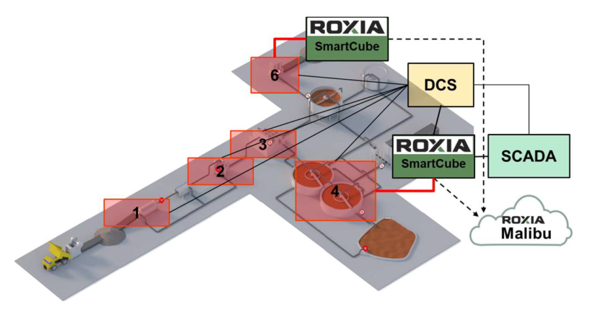
To extract the data from the filtration system, the SmartCube® reads directly from the PLC and from the DCS system of the plant. It is worth mentioning that the SmartCube® was installed based on a unidirectional communication premise. It is not possible to write data back to the equipment nor the DCS.

The read data is then preprocessed to make them ML-friendly, that is data are aggregated, cleanse, and arranged to be sent to the Malibu® cloud. These operations are explained in the following sections0.

We were interested to access data collected by the filters PLCs and auxiliary equipment gathered by external systems and presented in the DCS. Data from a total of 3740 cycle were used in this study.

It is widely known within the data science community that any endeavor dealing with data driven modeling has one major resource consumer, and activity that can occupy more than 50% of the time employed to generate and test these models, that is, preparing the collected data.

The data comes to the SmartCube® as time-series data. This is data that can be represented on a value vs. time reference system. As the data is collected under different frequency intervals, measures to correlate different collection instances (times) are a must and is here where the data manipulation algorithms running in the SmartCube® excel.

To describe the apparent arbitrariness in the data collection procedure, it is important to classify the type of data gathered. The first type of data collected that we deal with are those which are not bind to the cycle of the filter itself, e.g., the density of the slurry or the level of a tank. We called this data, cycle-independent data. Within these data, the collection frequency was selected according to the velocity of the changes on the variable studied. Three schemes were put in place to cover the full range of the nature of the data. We had time-based collection, on-change collection, and a hybrid of the time and on-change schemes.

Time-based collection schemes are defined as collecting data at a prescribed time interval, i.e., frequency. Every second, or every five seconds are examples of this collections scheme.

The collection frequency depends on the dynamic nature of the measured variable. For example, changes in the slurry density are assumed to be slower than changes on the flow of a pump. Hence, it is logic that lower collection frequencies are assigned to slowly changing variables.

On-change schemes means that the data is only collected after a changed is perceived. The SmartCube® is continuously monitoring the variable but only collects it when a change has occurred. Examples of these type of measurement could be closing or opening a valve.

The third collection scheme prioritizes when to collect the data under a “what occurs first” reasoning. A collection frequency is setup to instruct the SmartCube® to collect the value according to a defined interval unless a change occurs in-between which triggers the collection of the value.

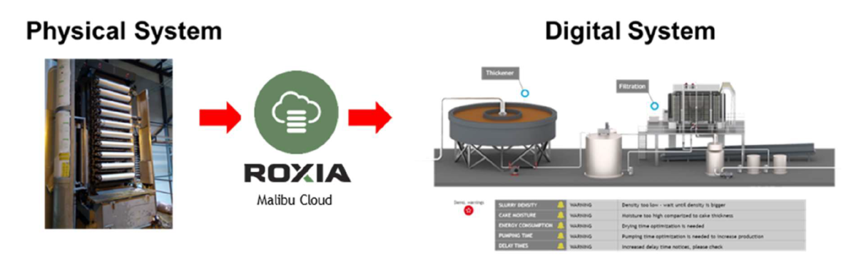
Data from three pressure filters were collected and the whole system was digitalized using the Roxia proprietary system Malibu® . These filters are part of a zinc concentration plant in Finland. Figure 3 presents a schematic of the digitalization created in the Malibu® system.

Malibu® reads approximately 200 data variables from each filter with variable collection frequency depending on the type of variable read. As an example, changes in the recipe stages are collected when the change occurs, while variables such as pressure and flow are collected every second. From the 200 variables, about 39 variables were selected to be used in the optimization algorithms as these variables were not related to alarms or valve open/close positions nor motors on/off status.

Different Machine Learning algorithms have been applied to optimize industrial processes [6]. In fact, from the wealth of research in the area, one might conclude that there is not a unique algorithm that could be applied universally to create industrial optimization routines. There are some most popular than other, such as Neural Networks [7]. However, for each case, researchers must pay close attention to details to select the algorithm able to describe the phenomena at hand. Within this successful group, Evolutionary Genetic Algorithms (EGA) have proven to give satisfactory answers to optimization problems postulated in the industry.

EGAs are machine learning algorithms that borrow from nature. These algorithms perform probabilistic search within the solution space based on what nature does to thrive as better generations appear one after another [8]. Each generation is produced by a series of common genetic operations such as random selection, survival of the bests, and mutation, among others. There exist extensive literature describing how newer generations are formed and what are the criteria to compose them. One of these evolutionary strategies is the µ + λ strategy [9]. The general process of a EGA cycle is presented in Figure 4.

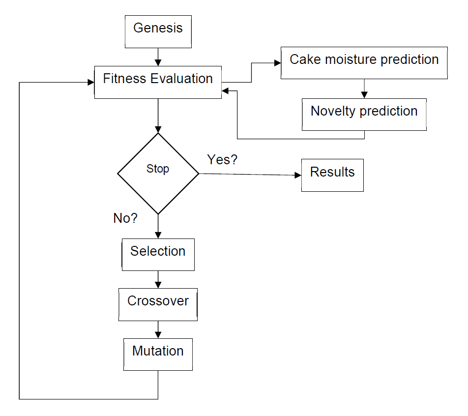
At the start of the optimization process, EGA model produces and aleatory population of 500 individuals filled with values of the features that can be controlled in the filtration process and are inherent to the filtration recipe, i.e., those parameters typically changed when adjusting the filter recipe. In this theoretical experiment the measured variables slurry flow, Drying air flow, pressure during pressing stage, wash water volume, filtration run time, second pressing run time and air-drying run time were used as optimizable parameters in the EGA’s routines.

Then, these set of values or genesis generation is tested against a scorer, which is heavily driven by the resulting cake moisture of the cake at the end of the cycle, cycle duration, and air consumption. Results are combined into a fitness equation to select the best actors in the current generation.

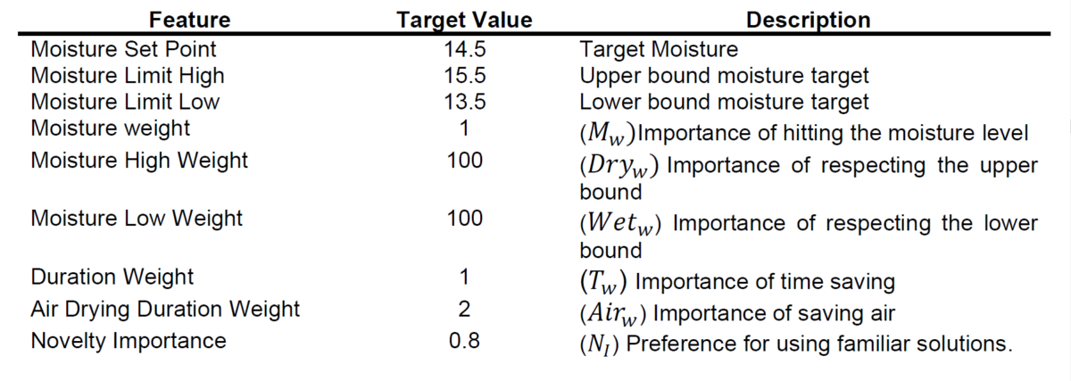
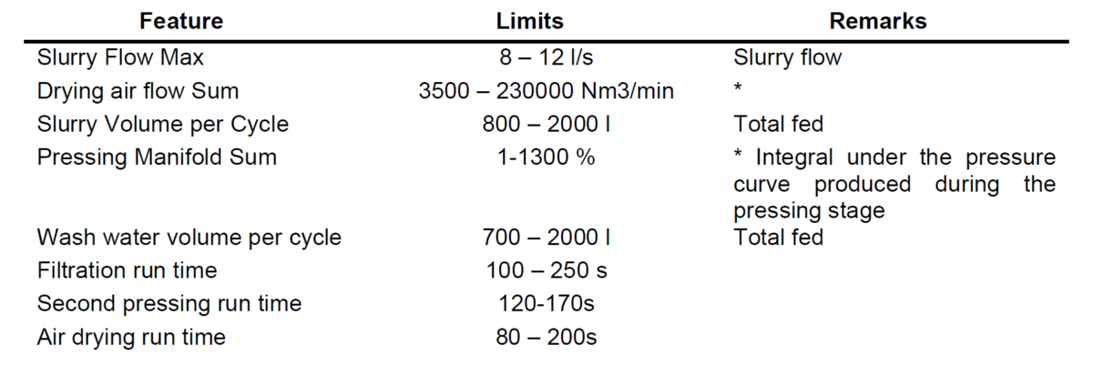
To create a scoring method for the filter optimizer, constraints and weights must be imposed on the target objectives (cake moisture, cycle duration, and drying air consumption). Table 1 and 2 presents the optimization targets and constraint used in this experiment.

To account for all the constraints and optimization targets, the following fitness function was
used. See equation (1)

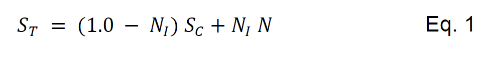
Where S் is the total score of the individual, and S஼ is the partial score resulting from meeting
the optimization targets as presented in equation (2).

In equation (2), Mௌ is the Moisture score defined by the square of the difference between the predicted moisture and the target value, Dry௉ is the penalty score resulting from squaring the differences between the upper deviation of the predicted moisture and the
upper bound moisture target. Similarly, Wet௉ is the corresponding penalty score in the lower bound. T௉ is the total cycle time of the individual. Finally, Air௉ is the air-drying flow penalty defined by the time taken in the drying stage.

The Novelty importance Nூ, comes from comparing the individual solution recipe with the solutions found in the collected data. We measure the probability of the individual solution to belong to the collected data distribution considering the collected data as an empirical cumulative distribution function.

After having the results of the fitness function per individual in the generation, an evolutionary strategy is applied. The next generation is formed by applying a μ + λ evolutionary strategy that takes the best actors of the parent generation and replaces 25% of it. Then, the rest of the members of the children generation are created by crossover and mutation of the individuals of the parent generation.

The new generation is then subjected to the fitness function again up to 100 generation have completed the loop. After these 100 generations, results are presented.

During the execution of the optimization routines, the optimizer is not only bounded to use real physical values in the variable space imposed by the mechanics of the filter. For example, the optimizer is constrained to use air flow values that do not exceed the maximum attainable air-drying flow of the studied equipment which comes from a limit set by the air compressor and piping system of the site. The optimizer it is also required to seek for solutions that comply with the expected quality of the cake represented by the cake moisture. This presents a challenge in many sites where there is not a reliable measurement of the cake moisture.

During this study, this challenge became evident when the cake moisture measurement instrument failed during the data collection period and only laboratory data was available. After analyzing the data collected manually and processed by the site laboratory, it was found that lab results were difficult to associate with a particular equipment and the value of the reported cake moisture variated amply. Not being able tie a value a specific filter automatically rendered the data unusable as it could not be set as feature for optimization purposes.

This challenge created an opportunity to develop and test a cake moisture prediction tool. Basically, a sub-product needed by the optimization tool. This prediction tool will take data generated during the filtration cycle to predict the resultant cake moisture at the end of that same cycle. A soft or virtual sensor was put in place as a redundant instrument to the physical one. This is not the first time virtual sensors have been used to back up physical sensors. There are many examples in the literature where virtual sensors came to solve issues related to difficulty of physical measurement of the variable, cost, and reliability of the physical instrument [10, 11].

As prediction tool, the research team used the Random Forest (RF) algorithm. The RF algorithm is a combination of simple decision trees algorithms such that each tree depends on the values of a random vector sampled independently and with the same distribution for all trees in the forest [12].

The RF algorithm is typically used as a classification algorithm in Machine learning. However, this algorithm has proven to be applied to a wide range of prediction problems
[13]. The advantage of using the RF algorithms is that is has only a few parameters to tune, and it is good to deal with small sample sizes and high-dimensional feature spaces [13]. The main requirement is to transform the problem into a supervised learning problem.

The RF has grown in popularity since its introduction in 2001. There exist a wealth of guided applications and research explaining the implementation of such versatile algorithm. Hence, in this paper, there are not explicit explanations of the theoretical foundations of the algorithm. During the study, we only the tuned the RF parameters to obtain an acceptable prediction accuracy. We invite the readers to investigate the RF algorithm implementation individually.

The application of any supervised machine learning algorithm such as the RF involves a series of steps to generate a useable model. After collecting the data, the RF model is trained. These basic steps are presented in Figure 5.

In the exploratory data analysis step, early conclusions on correlation of variables, commonalities of outliers and clear variable patterns, further data aggregation, and data splitting are carried out. In this step, the time-series data is also arranged to meet the requirements of a supervised learning problem. Features are outlined and domain expertise is used to weight initial feature importance subjectively. Clear examples of selection of relevant features can be seen in [14]

In the model training step, date is split into training and testing datasets. It is typical to find in the literature split ratios of 70-80 for training data set and 20-30 for the testing set and it is not uncommon to find a subdivision within the training dataset into training and validation sets [15]. In this research, an additional step was taken to reduce the bias and prevent overfitting of the RF prediction process. This additional step is widely known as cross
validation where data is resampled to estimate the true prediction error and to tune model parameters [16].

Cross-validation consist in splitting the whole set into smaller subsets with their own train and test sets. These sub-sets are then trained and tested in the model to get in each one of the train/testing rounds a measure of fitness in prediction of the outcome. These measures are then combined to obtain a more accurate estimate of the model performance. In this study the Scikit-learn python library was used [17]. Scikit has a helper function – cross_val_score- that allows the user to perform cross-validation and training and testing in one step. The tuning parameters in the cross_val_function was left with their default values.

To train and test the cake moisture prediction model, Scikit provides the function sklearn.ensemble.RandomForestRegressor, also with a series of tunable parameters to improve the accuracy of the model. The parameters tuned in this study and their values are shown in

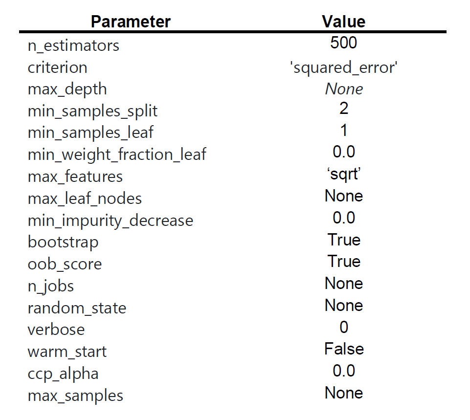
The evaluation of the model is done using an accuracy scoring method. All tests were assessed using the coefficient of determination R2 which corresponds to the proportion of the variance explained by the variables in a regression model. The highest the value of R2, the more accurate the model is.

To make accessible the resulting model to all the equipment, a cloud RESP API service was developed and deployed in Roxia’s Malibu® cloud. A server running a Python Flask application contained all the endpoints to receive data from the filters and return moisture
results to the on-site system.

At this stage of the development of the prediction tool, retrain routines were not implemented mainly due to the experimental nature of this research. However, retrain needs could be assessed by measuring drift and robustness of the model [18].

Not all variables collected from the filtration process contribute equally to predict accurately the cake moisture nor they are necessary. This is a challenge that many multivariate problems have. Recognizing the a priori importance of certain variables might be guided by information gathered from physical models and experience. However, it is not guaranteed that the variables or features selected will be enough to get high accuracy or describe the phenomena.

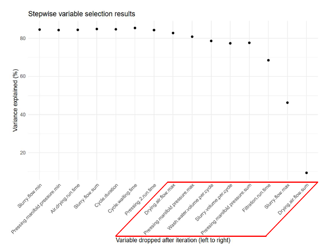
Out of the 39 variables collected per filter, it can be expected that just a few of them will explain the behavior of the cake moisture at the end of the cycle. To reduce the dimensionality of the prediction problem a backward feature selection scheme was used [19, 20]. A sequential backward selection algorithm is constructed by starting with a full set of features in the first training trial. Then, one feature at a time is removed testing whose removal gives the lowest decrease in predictor performance.

The results of processing these 3740 filtration cycles are presented in different order to that shown in the methods section. First, the results of the cake moisture prediction tool are discussed together with the feature selection routine outcomes. Then, results from the application of the EGA are presented.

The results of the cake moisture prediction are first presented as correlation charts in Figures Figure 6, 7, and 8 for filters 1, 2, and 3. These correlation charts plot the predicted moisture content versus the moisture measured by the physical sensor. The physical measurement is considered the real moisture of the cake although it can be argued that errors and averaging in the measuring process can tremendously affect this value.

It can be notably seen the difference in number of measurements for each filter. This difference occurred because during the data collection process, filters 2 and 3 were predominantly used. It can be observed also that the variation on moisture contented of the different filters is different. Filter 1 produced more accurate cakes consistently than the other two filters although the differences did not exceed ±1.5 percentual points from the target cake moisture.

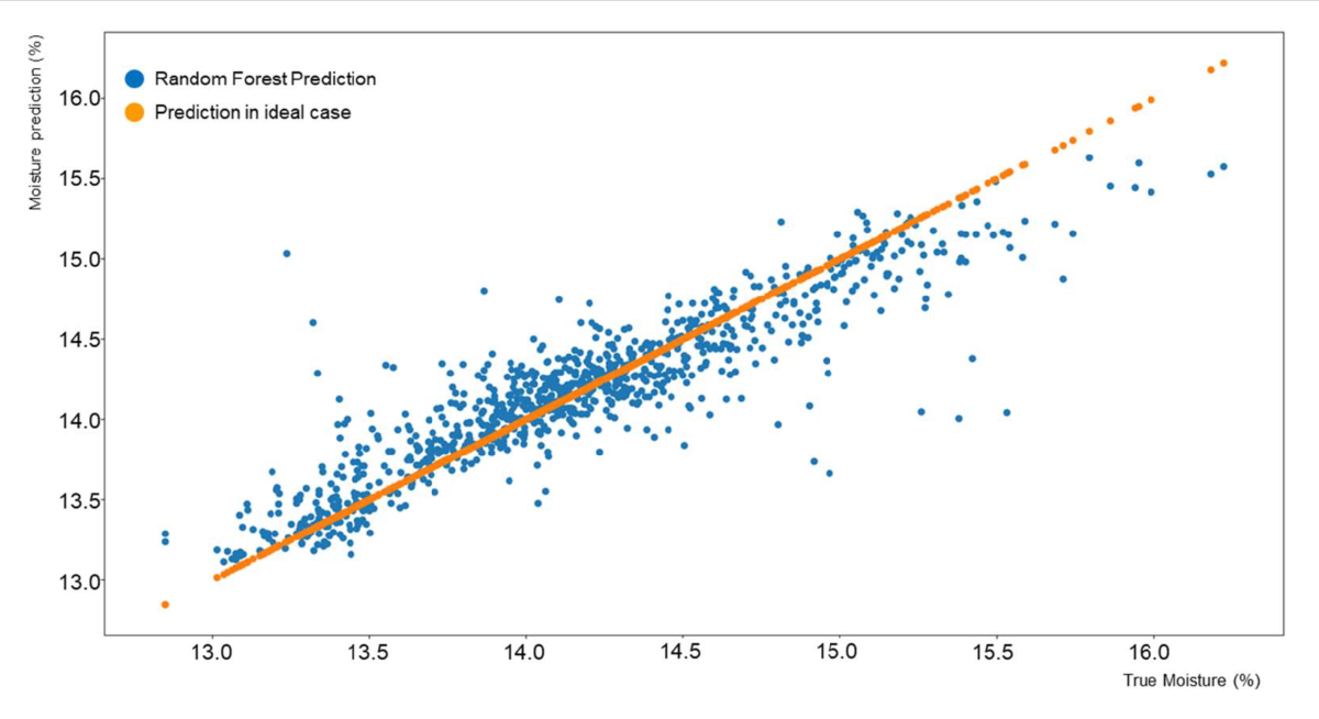
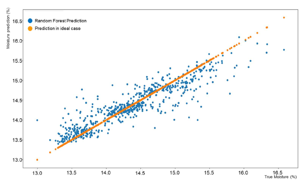
In general, results from the prediction process were in the 95% confidence interval which was about 0.9% units wide. This means that a predicted moisture of 15.21% would have confidence bounds of [14.81, 15.72]. For the current data set, in 95% of the cases the true values will be within ±0.45 units from the predicted value.

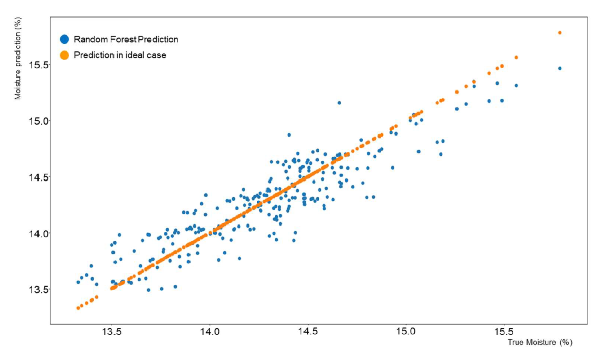
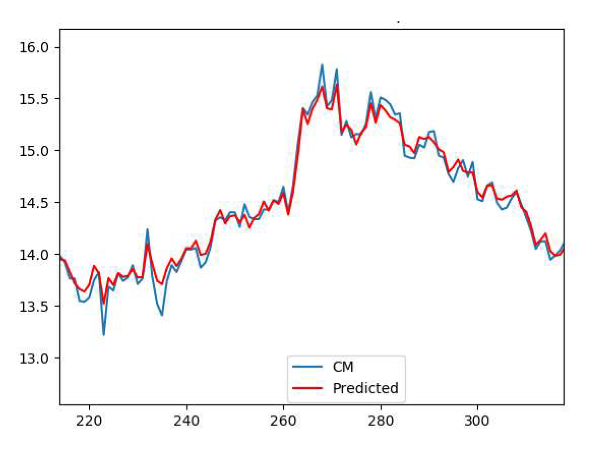
Next, the trained cake moisture prediction tool was independently run continuously to verify prediction results on 500 cycles. Figure 9 presents the results of the application of the prediction tool to these cycles. It can be seen how close the predicted value was from the true value during the trials. It is important to mentioned that overfitting of the predictor is a possibility. However, by looking at the results of the optimization routine, as it will be seen in the next section, the fact that close to 70% of the optimizer solutions fell withing a known set of familiar solutions might explain the behavior.

All 39 collected variables did not contribute to the accuracy of the prediction model. After applying the sequential backward selection model, eight features became evident responsible for the success in the prediction of the cake moisture. These variables were also used as part of the controllable variables tuned in the filter recipe optimization process. Figure 10 shows the eight important variables to predict the cake moisture in the Random
Forest model.

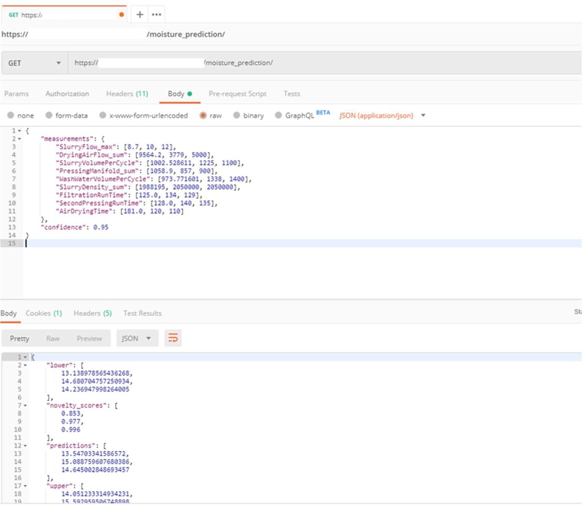
Data from a completed cycle is sent via GET request to the prediction model running in the Roxia cloud. Figure 11 shows a snapshot of one of the requests to the prediction model. In the case presented in the figure, information from three cycles was sent in one request. This means that these transactions can be performed on an array of values and they will return an array of solutions of the same length.

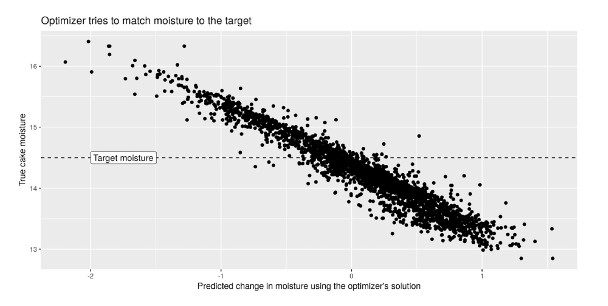
One interesting behavior found in the optimizer was that it tried to enforce the target moisture of the cake. The design of the optimizer tended to produce dryer cakes. The tendency can be seen in Figure 12. Note how results concentrated below the target moisture setup in the constraints of the model. Interesting also to notice is that although wetter and dryer cakes had the same penalty factors, the optimizer pushed the solution towards the dry side.

Novel solutions, those with novelty score > 95% seemed to provide shorter cycle durations
than familiar solutions. This can be observed in Figure 13.

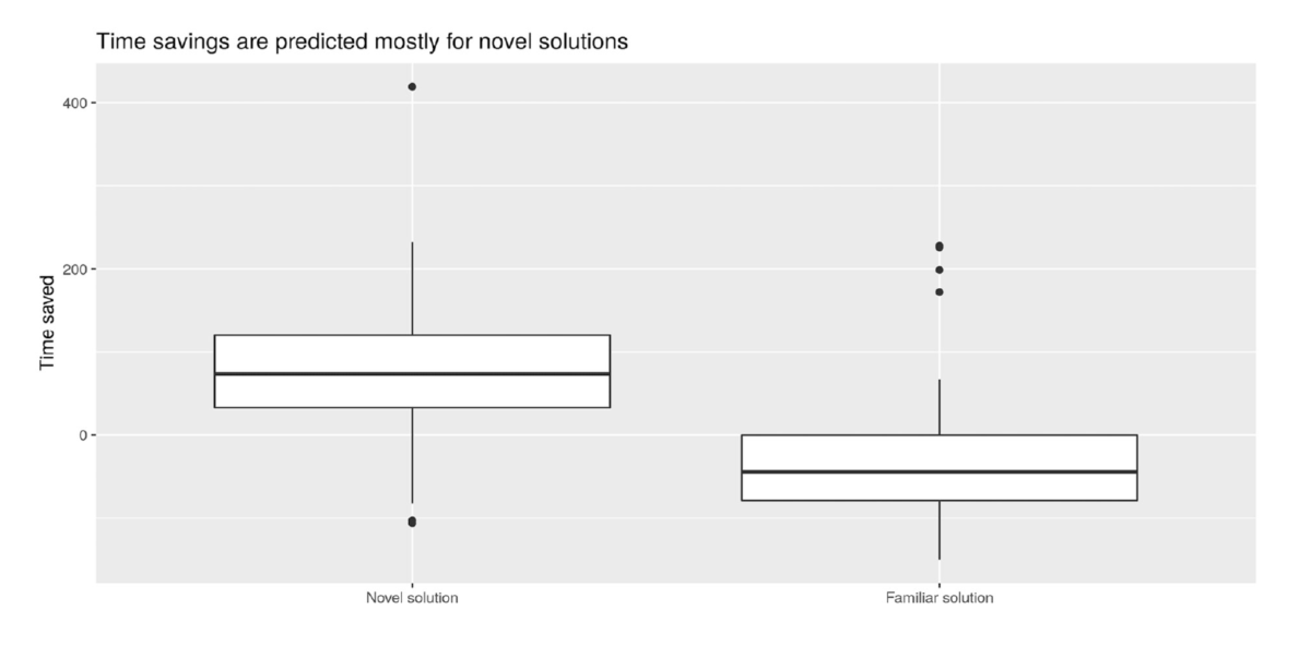
Solutions for the time savings had a median of 80 seconds with values for the 25th and 75th percentile of 40 – 120 seconds, respectively. Minimum and maximum values were in the order of -85 to 240 seconds.

Looking at the changes proposed by the optimizer in its novel solutions, a few interesting points could be argued. From Figure 14 can be seen that novel solutions propose reducing air-drying time while increasing air flow. Then, aiming at reducing the air consumed during the filtration cycle might seem not reachable with the current configuration.

Regarding filtration run time, novel solutions are more scatter over the variation suggested or achieved by the familiar solutions. However, there was an important presence of novel solutions recommending reducing the filtration time.

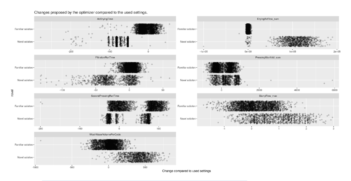
Pressure applied during the pressing stage did not seem to be much different from the familiar to the novel solutions. The same behavior was also seen for the second pressing stage run time. Although, it is worth commenting that novel solutions for he second pressing run time were more concentrated that the familiar solutions.

Not much variation was suggested in the maximum slurry flow fed to the filter. However, novel solutions suggested using more washing water.

This theoretical work on data-driven optimization and prediction has resulted in clear signs that such data-driven approaches could be used to improve the operation of a filtration process. As has been stated in different studies, pressure filtration is still a complex topic to be completely defined by a unique physical model. Yet, undoubtedly the increasing physical knowledgebase on filtration keeps adding pieces to the big puzzle filtration seems to be. It
is not the intention of the team to suggest that data-driven models could replace completely physical models. We think that there is a bigger picture were both worlds could be combined to produce better results and advances in the field.

Originally, our intention was to dynamically adjust the steps of the filtration cycle as they were occurring. However, at this early stage, we didn’t find enough stage-intermediate variable measurement to follow this approach as certain data were collected only after the cycle had finished. This could be part of an interesting future study where the filter really adjusts in real-time its recipe taking information from the same running cycle.

Suggestions to change filtration recipes given by the EGA optimizer were based on the initial assumption that from one cycle to next, there were not radical changes of the characteristics of the slurry. According to the obtained results, neither the optimizer nor the cake moisture predictor needed to be retrained due to drifting and changes in the robustness of their solution. We expect that changes would indeed occur with time and a good complement to this research could be using previous slurry characterization studies as a preparatory step for the optimization process. Researchers have studied ways to describe slurry characteristics in the past [21]. Implementing their findings in future studies to optimize filtration cycles is recommended as future work.

For the 3740 cycles studied, it was found that the optimization routing was able to find cycle time savings between 40 seconds and 2 minutes. These can correspond to savings in the order of 3 – 12.5% in a filter with a typical filter cycle duration of 16 minutes. In one of the seminal works in filtration cycle optimization, the approximate cycle time reduction was about 12% following simulations based on physical models [4]. We are confident that data
driven models can produce better results if more thought could be given to what type of extra instrumentation might be useful to collect data that is non existing in this study. One example could be data from particle size distribution of the slurry.

From the optimization results, it was shown that out of the optimal solutions 29% could be considered novel, that is, those solutions with a novelty score > 95%. This means that these type of settings or recipes were not found in the training data but were obtained using extrapolation.

These novel solutions involved changes such as decreasing air-drying time but at the expense of increased air flow. We can argue that a better a fitness function could be used where minimizing air flow could be added as constraint to the problem. Other changes that appear were decreased filtration run time, increased second pressing runt time, increased slurry flow and increased wash water volume.

In the case of the cake moisture prediction tool used as sub-module of the EGA optimization routine, it was found that the variables that essentially explain cake moisture in this study are related to how much pressure was applied, how much water and slurry were used, and how much air was used in drying. This tool was able to predict cake moisture with a 95% of confidence translating into a confidence interval of 0.9% units of difference with respect to the real measurement.

Models and algorithms were tested in the Roxia cloud environment. A server running a Python application received GET and POST API with the data collected from the Malibu® system. Then, the data was used in the EGA and prediction tool models to give filter recipe suggestions. The maximum latency found to get a response from the cloud from the moment of emitting the GET or POST request was about 10s. It means that after a cycle is finalized the equipment could get in an average of 10s new instructions for the next cycle.

The team at Roxia would like to thank Business Finland for funding this research.

[1] T. XU, Q. ZHU, X. CHEN and W. LI, “Equivalent Cake Filtration Model,” Chinese Journal of Chemical Engineering, vol. 16, no. 2, pp. 214 – 217, 2008.

[2] C. Visvanathan and R. Ben Aim, Water, Wastewater, and Sludge Filtration, CRC Press, 1989.

[3] S. Jämsä-Jounela, J. S. Tóth, M. Oja and K. Junkarinen, “MODELLING MODULE OF THE INTELLIGENT CONTROL SYSTEM,” Automation in Mining, Mineral and Metal Processing, 1998.

[4] S. Jämsä-Jounela, M. Vermasvuori and K. Koskela, “Operation Cycle Optimization Of The Larox Pressure Filter,” Cost Oriented Automation, 2004.

[5] S. Jämsä-Jounela, M. Vermasvuori, J. Kämpe and K. Koskela, “Operator support system for pressure filters,” Control Engineering Practice, vol. 13, pp. 1327-1337, 2005.

[6] D. Weichert, P. Link, A. Stoll, S. Rüping, S. Ihlenfeldt and S. Wrobel, “A review of machine learning for the optimization of production processes,” The International Journal of Advanced Manufacturing Technology, vol. 104, pp. 1889-1902, 2019.

[7] M. Bertolini, D. Mezzogori, M. Neroni, Zammori and F, “Machine Learning for industrial applications: A comprehensive literature review,” Expert Systems With Applications, vol. 175, pp. 1-29, 2021.

[8] D. Goldberg and J. Holland, “Genetic Algorithms and Machine Learning,” Machine Learning, vol. 3, pp. 95-99, 1988.

[9] A. Slowik and H. Kwasnicka, “Evolutionary algorithms and their applications to engineering,” Neural Computing and Applications, vol. 32, p. 12363–12379, 2020.

[10] S. Kabadayi, A. Pridgen and C. Julien, “Virtual Sensors: Abstracting Data from Physical Sensors,” in International Symposium on a World of Wireless, Mobile and Multimedia Networks(WoWMoM’06), 2006.

[11] K. Manabu and F. Koichi, “Virtual Sensing Technology in Process Industries: Trends and Challenges Revealed by Recent Industrial Applications,” JOURNAL OF CHEMICAL ENGINEERING OF JAPAN, vol. 46, no. 1, pp. 1-17, 2013.

[12] L. Breiman, “Random Forests,” Machine Learning, no. 45, pp. 5-32, 2001. [13] G. Biau and E. Scornet, “A random forest guided tour,” Test, no. 25, pp. 197-227, 2016.

[14] L. Avrim and P. Langley, “Selection of relevant features and examples in machine learning,” Artificial Intelligence, vol. 97, no. 1–2, pp. 245-271, 1997.

[15] S. A. Raykar V.C., “Data Split Strategiesfor Evolving Predictive Models.,” in Appice A., Rodrigues P., Santos Costa V., Soares C., Gama J., Jorge A. (eds) Machine Learning and Knowledge Discovery in Databases. ECML PKDD 2015., 2015.

[16] D. Berrar, “Cross-Validation,” Encyclopedia of Bioinformatics and Computational Biology, vol. 1, pp. 542-545, 2018.

[17] F. e. a. Pedregosa, “Scikit-learn: Machine learning in Python,” Journal of machine learning research, no. 12, p. 2825–2830, 2011.

[18] A. Kavikondala, V. Muppalla, K. Prakasha and V. Acharya, “Automated Retraining of Machine Learning Models,” International Journal of Innovative Technology and Exploring Engineering, vol. 8, no. 12, pp. 445-452, 2019.

[19] G. Chandrashekar and F. Sahin, “A survey on feature selection methods,” Computers & Electrical Engineering, vol. 40, no. 1, pp. 16-28, 2016.

[20] F. Ferri, P. Pudil and M. Hatef, “Comparative Study of Techniques for Large-Scale Feature Selection,” Pattern Recognition in Practice, IV: Multiple Paradigms, Comparative Studies and Hybrid Systems, vol. 16, 2001.

[21] S. Laine, H. Lappalainen and S. Jämsä-Jounela, “On-line determination of ore type using cluster analysis and neural networks,” Minerals Engineering, vol. 8, pp. 637- 6348, 1995.

[22] G. Louppe, L. Wehenkel, A. Sutera and P. Geurts, “Understanding variable importances in Forests of randomized trees,” in NIPS 2013, 2013.